Alignment

• find parameters of model that maps one set of points to another
• Typically want to solve for a global transformation that accounts for most true correspondence

Difficulties

• Noise (typically 1-3 pixels)
• Outliers (often 50%)
• Many-to-one matches or multiple objects

Parametric (global) warping

• Transformation T is a coordinate-changing machine: $p' = T(p)$
• T is global
• global :
  • Is the same for any point p
  • can be described by just a few numbers (parameters)
• For linear transformations, we can represent T as a matrix

$\begin{bmatrix} x'\\ y' \end{bmatrix} = T\begin{bmatrix} x\\ y \end{bmatrix}$

Scaling

Scaling a coordinate means multiplying each of its components by a scalar

• Uniform scaling means this scalar is the same for all components:
• Non-uniform scaling: different scalars per component

operation :

• $x' = ax$
• $y' = by$

matrix form :

• $\begin{bmatrix} x'\\ y' \end{bmatrix} = \begin{bmatrix} a & 0\\ 0 & b \end{bmatrix} \begin{bmatrix} x\\ y \end{bmatrix}$

2-D Rotation

• operation :
  • $x' = x \text{cos}(\theta) - y \text{sin}(\theta)$
  • $y' = x \text{sin}(\theta) - y \text{cos}(\theta)$
• matrix form :
  • $\begin{bmatrix} x'\\ y' \end{bmatrix} = \begin{bmatrix} \text{cos}(\theta) & -\text{sin}(\theta)\\ \text{sin}(\theta) & \text{cos}(\theta) \end{bmatrix} \begin{bmatrix} x\\ y \end{bmatrix}$
• Even though sin($\theta$) and cos($\theta$) are nonlinear functions of $\theta$
  • x’ is a linear combination of x and y
  • y’ is a linear combination of x and y
• What is the inverse transformation?
  • rotation by $-\theta$
  • for rotation matrices $R^{-1} = R^T$

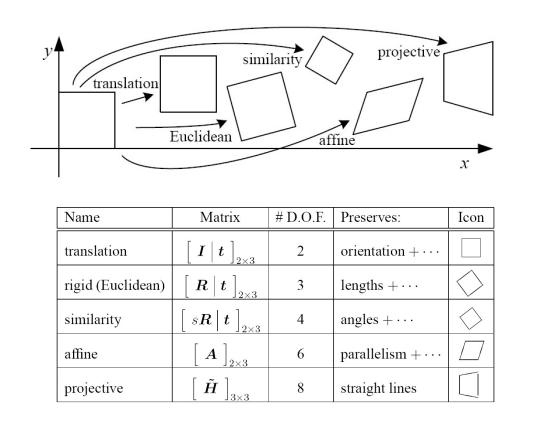
Basic 2D transformations

• scale $\begin{bmatrix} x'\\ y' \end{bmatrix} = \begin{bmatrix} s_x & 0\\ 0 & s_y \end{bmatrix} \begin{bmatrix} x\\ y \end{bmatrix}$
• shear $\begin{bmatrix} x'\\ y' \end{bmatrix} = \begin{bmatrix} 1 & \alpha_x\\ \alpha_y & 1 \end{bmatrix} \begin{bmatrix} x\\ y \end{bmatrix}$
• rotate $\begin{bmatrix} x'\\ y' \end{bmatrix} = \begin{bmatrix} \text{cos}(\theta) & -\text{sin}(\theta)\\ \text{sin}(\theta) & \text{cos}(\theta) \end{bmatrix} \begin{bmatrix} x\\ y \end{bmatrix}$
• translate $\begin{bmatrix} x'\\ y' \end{bmatrix} = \begin{bmatrix} 1 & 0 & t_x\\ 0 & 1 & t_y \end{bmatrix} \begin{bmatrix} x\\ y\\ 1 \end{bmatrix}$
• affine $\begin{bmatrix} x'\\ y' \end{bmatrix} = \begin{bmatrix} a & b & c\\ d & e & f \end{bmatrix} \begin{bmatrix} x\\ y\\ 1 \end{bmatrix}$ or $\begin{bmatrix} x'\\ y'\\ 1 \end{bmatrix} = \begin{bmatrix} a & b & c\\ d & e & f\\ 0 & 0 & 1 \end{bmatrix} \begin{bmatrix} x\\ y\\ 1 \end{bmatrix}$

Affine Transformations

Affine transformations are combinations of

• Linear transformations
• Translations

Properties of affine transformations:

• Lines map to lines
• Parallel lines remain parallel
• Ratios are preserved
• Closed under composition

Projective(perspective) Transformations

$\begin{bmatrix} x'\\ y'\\ w' \end{bmatrix} = \begin{bmatrix} a & b & c\\ d & e & f\\ g & h & i \end{bmatrix} \begin{bmatrix} x\\ y\\ w \end{bmatrix}$

Projective transformations are combos of

• Affine transformations, and
• Projective warps

Properties of projective transformations:

• Lines map to lines
• Parallel lines do not necessarily remain parallel
• Ratios are not preserved
• Closed under composition
• Models change of basis
• Projective matrix is defined up to a scale (8 DOF)

Example: solving for translation

1. Least squares solution

   Problem: outliers

2. RANSAC solution

   Problem: outliers, multiple objects, and/or many-to-one matches

3. Hough transform solution

   Problem: no initial guesses for correspondence

Iterative Closest Points (ICP) Algorithm

If we don’t have initial alignment

estimate transform between two dense sets of points

1. Initialize transformation (e.g., compute difference in means and scale)
2. Assign each point in Set 1 to its nearest neighbor in Set 2
3. Estimate transformation parameters
   • e.g., least squares or robust least squares
4. Transform the points in Set 1 using estimated parameters
5. Repeat steps 2-4 until change is very small