recognition tasks

• Scene caategorization / classification
  • outdoor / indoor
  • city / forest / factory / …
• Image annotation / tagging / attributes
  • street / people / building / mountain / tourism / cloudy / brick
• Object detection
  • find pedestrians
• Image parsing / semantic segmentation
  • sky / mountain / building / tree
• Scene understanding

History of ideas in recognition

• 1960s – early 1990s: the geometric era

  • Recognition as an alignment problem : Block world Invariant to
    • Camera position
    • Illumination
    • Internal parameters
  • Recognition by components
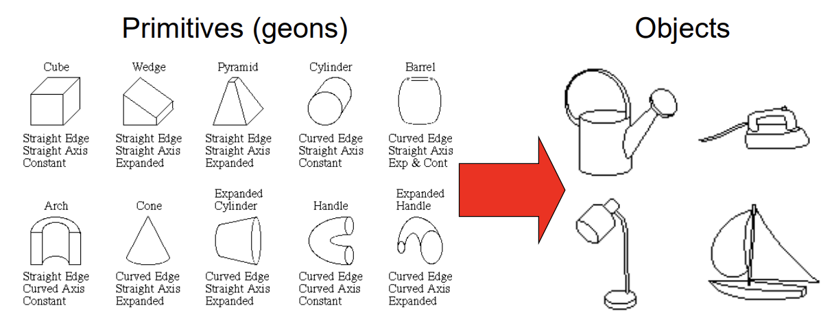
    • rigid Zisserman et al. (1995)
    • non-rigid Zisserman et al. (1995)

• 1990s: appearance-based models

  Eigenfaces

  (Turk & Pentland, 1991)

  Color Histograms

  

  Appearance manifolds

  feature space

  Limitations of global appearance models

  global appearance model : entire image → feature vector

  • Requires global registration of patterns
  • Not robust to clutter, occlusion, geometric transformations translation will affect the whole feature vector

• Mid-1990s: sliding window approache

  Sliding window approaches

• Late 1990s: local features

  Large-scale image search

  

• Early 2000s: parts-and-shape models

  Parts-and-shape models

  • Object as a set of parts
  • Relative locations between parts
  • Appearance of part

  Constellation models

  Pictorial structure model

  Discriminatively trained part-based models

  gradient orientation

• Mid-2000s: bags of features

  Bag-of-features models

  object → bag of words

  Objects as texture

  Origin 1: Texture recognition

  • Texture is characterized by the repetition of basic elements or textons
  • For stochastic textures, it is the identity of the textons, not their spatial arrangement, that matters Origin 2: Bag-of-words models

  step

  1. Extract features

     1. detect patch
        • Regular grid
        • Interest region
     2. normalize patch
     3. compute descriptor

  2. Learn “visual vocabulary”

     

     descriptor -clustering-> keyword

     visual vocabulary = set of keyword

     K-means clustering

     • Want to minimize sum of squared Euclidean distances between points $x_i$ and their nearest cluster centers $m_k$ $D(X, M) = \sum_{\text{cluster} k}\sum_{\text{point} i \text{in cluster} k}(x_i - m_k)^2$
     • Algorithm
       • K개의 클러스터 센터를 랜덤하게 초기화
       • 수렴할 때까지 다음을 반복
         • 각 데이터를 가장 가까운 중심에 할당함
         • 각 클러스터 센터를 할당된 모든 점의 평균으로 다시 계산

  3. Quantize features using visual vocabulary

     Clustering and vector quantization

     • Clustering is a common method for learning a visual vocaburary or codebook
       • (partially) Unsupervised learning process
       • Each cluster center produced by k-means becomes a codevector
       • Codebook can be learned on separate training set
       • Provided the training set is sufficiently representative, the codebook will be “universal”
     • The codebook is used for quantizing features
       • A vector quantizer takes a feature vector and maps it to the index of the nearest codevector in a codebook
       • Codebook = visual vocabulary
       • Codevector = visual word
     • Example codebook

  4. Represent images by frequencies of “visual words”

  Visual vocabularies: Issues

  • vocabulary size
    • too small : visual words not representative of all patches / loose detail
    • too large : quantization artifacts / overfitting / computational overhead
  • computational efficiency → Vocabulary trees

  Spatial pyramid

  Extension of a bag of features Locally orderless representation at several levels of resolution coarse to fine matching

• ~2010s: combination of local and global methods, datadriven methods, context

  Global scene descriptors

  The “gist” of a scene

  Data-driven methods

  Geometric context

Face Detection

• Identification at a distance
• Easy to capture from low-cost cameras
• Non-contact acquisition (free from contagious disease)
• Covert acquisition (ubiquitous surveillance cameras)
• Legacy databases (passport, visa and driver license)

Knowledge-based methods

• Encode what constitutes a typical face, e.g., the relationship between facial features
• Pros
  • Easy to come up with simple rules
  • Based on the coded rules, facial features in an input image are extracted first, and face candidates are identified
• Cons
  • Difficult to translate human knowledge into rules precisely: detailed rules fail to detect faces and general rules may find many false positives
  • Difficult to extend this approach to detect faces in different poses: implausible to enumerate all the possible cases

Color based methods

• Use a color model, usually in HSV space
• Pros
  • Easy to implement
  • Insensitive to pose, expression, rotation variation
• Cons
  • Sensitive to environment and lighting change
  • High false positives

Template matching

• Several standard patterns stored to describe the face as a whole or the facial features separately
• Cross-correlation with a template
• Pros
  • Simple
• Cons
  • Difficult to enumerate templates for different poses and scales (similar to knowledge-based methods)

Feature based approaches:

• A set of features that describe each part of face region
• Learning-based approaches
  • Neural Nets [Rowley et al, PAMI 98]
  • SVMs [Heisele and Poggio, CVPR 01]
  • Boosting + Harr feature [Viola and Jones, ICCV 01]
  • Boosting + Edge Orientation Histogram [Levy & Weiss, 2004]
• General facial features: edge, intensity, shape, texture, etc
  • Haar feature (integral image)
• Aim to detect invariant features

Viola-Jones Face Detector

We can observe that a human face has some useful characteristics, for example:

• The area of eyes is usually darker than the area of the bridge of the nose
• The area across eyes is usually darker than the area of cheeks.

Four basic shape bases are used

• The white areas are subtracted from the black ones.
• A special representation of the sample called the integral image makes feature extraction faster

Sub-windows with different sizes starting from 24x24

Rectangle Integral Image (RII)

$RII(x, y) = \sum_{x' \leq x, y' \leq y}I(x', y')$

Weak classifier

AdaBoost algorithm

Strong classifier

Cascade of Strong Classifiers